- SpreadJS Overview
- Getting Started
- JavaScript Frameworks
- Best Practices
- Features
- SpreadJS Designer
- SpreadJS Designer Component
- Touch Support
-
Formula Reference
- Formula Overview
-
Formula Functions
- Barcode Functions
- Compatibility Functions
- Database Functions
- Date and Time Functions
- Engineering Functions
- Financial Functions
- Information Functions
- Logical Functions
- Lookup and Reference Functions
- Math and Trigonometric Functions
- Statistical Functions
- Sparkline Functions
- Text Functions
- Web Functions
- Other Functions
- RegEx Functions
- Import and Export Reference
- Frequently Used Events
- API Documentation
- Release Notes
XLOOKUP
XLOOKUP performs lookups in vertical and horizontal cell ranges and provides support for approximate matching, partial matching (using wildcard characters like *, ? etc.) and exact matching. By default, the XLOOKUP function returns the exact matched results.
The XLOOKUP function is comparatively more flexible and powerful than the rest of the lookup functions (like VLOOKUP, HLOOKUP, LOOKUP, etc.). Some more benefits of using the XLOOKUP function instead of other lookup functions are listed below:
Users can use the XLOOKUP function to lookup data to the right or left of the lookup values.
Users can use the XLOOKUP function to retrieve data from a table.
Users can return results from more than one column by using the XLOOKUP function.
The XLOOKUP function can work with both vertical and horizontal data.
The XLOOKUP function can also be used for searching data starting from the first value or the last value (reverse lookup).
The XLOOKUP function returns a range instead of just a value and can work with generic arrays as well.
For instance - By using the XLOOKUP function, users can determine the price of a product by its product ID, find a matching tax rate in a column, search an employee name based on their employee ID and perform many other search operations while working with spreadsheets.
Syntax
XLOOKUP(lookup_value, lookup_array, return_array, [if_not_found], [match_mode], [search_mode])
Arguments
This function has the following arguments:
Argument | Description |
|---|---|
lookup_value | Refers to the lookup value. |
lookup_array | Refers to the lookup array or cell range that you want to search. |
return_array | Refers to the array or cell range that you want to return. |
[if_not_found] | [Optional] Refers to the value to be returned when no match is found. If users don't specify this argument, and no matches are found, then the function returns the #N/A error. When users specify an invalid search mode (E.g. - 0 in Excel), then the #VALUE error will be returned. |
[match_mode] | [Optional] Specifies the type of the match as per the following values: 0 - Refers to exact match. If no matches are found, then the #N/A error is returned. This is the default match mode. -1 - Refers to exact match. If no matches are found, then the next smaller item is returned. 1 - Refers to exact match. If no matches are found, then the next larger item is returned. 2 - Refers to a wildcard match where "*", "?" and "~" characters possess special meanings to indicate a partial match. |
[search_mode] | [Optional] Specifies the mode of the search as per the following values: 0 - Refers to the "search all" mode where all the matched values will be returned. [This mode is not available in Excel.] 1 - Refers to a search that starts at the first item. This is the default search mode. -1 - Refers to a reverse search that starts at the last item. 2 - Refers to a binary search that depends upon the lookup_array argument being sorted in ascending order. -2 - Refers to a binary search that depends upon the lookup_array argument being sorted in descending order. |
not_found | [Optional] This argument can be used to override the #N/A error. Typical values for not_found might be "Not found", "No match", "No result", etc. |
Remarks
The following points must be kept in mind while working with the XLOOKUP function in the spreadsheets:
The XLOOKUP function returns the #N/A error if the lookup value is not found.
The dimensions of the lookup_array argument must be compatible with the return_array argument for a valid result, else the XLOOKUP function will return the #VALUE! error.
Data Types
Accepts numeric data. Looks up values in a range or table. Returns an array with multiple items.
Examples
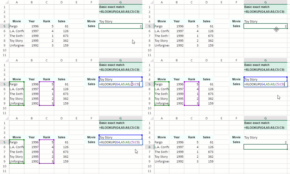
The following gif shows the basic usage of XLOOKUP function.

The following code snippet depicts the basic usage of XLOOKUP function. In this example, XLOOKUP is used to retrieve Rank based on an exact match on Movie.
$(document).ready(function () {
    // Initializing Spread
    var spread = new GC.Spread.Sheets.Workbook(document.getElementById('ss'), { sheetCount: 1 });
    // Enable dynamic array support
    spread.options.allowDynamicArray = true;
    // Create style
    var style = new GC.Spread.Sheets.Style();
    style.font = "bold 12px Arial";
    style.foreColor = "black";
    style.backColor = "#EDFDF4";
    style.hAlign = GC.Spread.Sheets.HorizontalAlign.center;
    style.vAlign = GC.Spread.Sheets.VerticalAlign.center;

    // Create style
    var formulaStyle = new GC.Spread.Sheets.Style();
    formulaStyle.font = "bold 12px Arial";
    formulaStyle.foreColor = "black";
    formulaStyle.backColor = "#D3F0E0";
    formulaStyle.vAlign = GC.Spread.Sheets.VerticalAlign.center;


    // Get the sheet1
    var sheet1 = spread.getSheet(0);
    // Set column width
    sheet1.setColumnWidth(6, 180);
    // Create formula
    var formula_Exact = '=XLOOKUP(G4,A5:A9,C5:C9)';
    // Set value
    sheet1.setValue(0, 6, 'Basic exact match');
    sheet1.setValue(1, 6, formula_Exact);
    // Create data
    var data = [
        ["Movie", "Year", "Rank", "Sales"],
        ["Fargo", 1996, 5, 61],
        ["L.A. Confidential", 1997, 4, 126],
        ["The Sixth Sense", 1999, 1, 673],
        ["Toy Story", 1995, 2, 362],
        ["Unforgiven", 1992, 3, 159]
    ];
    // Set data
    sheet1.setArray(3, 0, data);
    // Set value
    sheet1.setValue(3, 5, 'Movie');
    sheet1.setValue(4, 5, 'Sales');
    sheet1.setValue(3, 6, 'Toy Story');
    // Set formula
    sheet1.setFormula(4, 6, formula_Exact);

    // Set style
    for (var i = 0; i < 4; i++) {
        sheet1.setStyle(3, i, style, GC.Spread.Sheets.SheetArea.viewport);
    }
    sheet1.setStyle(3, 5, style, GC.Spread.Sheets.SheetArea.viewport);
    sheet1.setStyle(4, 5, style, GC.Spread.Sheets.SheetArea.viewport);
    sheet1.setStyle(0, 6, formulaStyle, GC.Spread.Sheets.SheetArea.viewport);
    sheet1.setStyle(1, 6, formulaStyle, GC.Spread.Sheets.SheetArea.viewport);
});
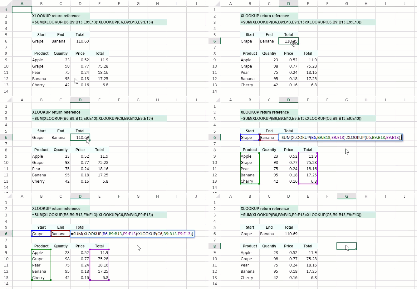
The following gif shows the SUM and XLOOKUP function works together to sum all the values between two ranges.

The following code sample shows how to use the SUM and XLOOKUP functions together.
$(document).ready(function () {
    // Initializing Spread
    var spread = new GC.Spread.Sheets.Workbook(document.getElementById('ss'), { sheetCount: 1 });
    // Enable dynamic array support
    spread.options.allowDynamicArray = true;

    // Get the sheet7
    var sheet7 = spread.getSheet(0);

    // Set text
    sheet1.setValue(1, 1, 'XLOOKUP return reference');
    sheet1.setValue(2, 1, '=SUM(XLOOKUP(B6,B9:B13,E9:E13):XLOOKUP(C6,B9:B13,E9:E13))');
    sheet1.addSpan(1, 1, 1, 3, GC.Spread.Sheets.SheetArea.viewport);
    sheet1.addSpan(2, 1, 1, 7, GC.Spread.Sheets.SheetArea.viewport);

    sheet1.setValue(4, 1, 'Start');
    sheet1.setValue(4, 2, 'End');
    sheet1.setValue(4, 3, 'Total');
    sheet1.setValue(5, 1, 'Grape');
    sheet1.setValue(5, 2, 'Banana');

    // Create data
    var data = [
        ["Product", "Quantiy", "Price", "Total"],
        ["Apple", 23, 0.52, 11.9],
        ["Grape", 98, 0.77, 75.28],
        ["Pear", 75, 0.24, 18.16],
        ["Banana", 95, 0.18, 17.25],
        ["Cherry", 42, 0.16, 6.8]
    ];
    // set data
    sheet7.setArray(7, 1, data);
    // set formula
    sheet7.setFormula(5, 3, "=SUM(XLOOKUP(B6,B9:B13,E9:E13):XLOOKUP(C6,B9:B13,E9:E13))");

    // set style
    for (var i = 1; i < 5; i++) {
        sheet7.setStyle(7, i, style, GC.Spread.Sheets.SheetArea.viewport);
    }
    for (var i = 1; i < 4; i++) {
        sheet7.setStyle(4, i, style, GC.Spread.Sheets.SheetArea.viewport);
    }
    sheet7.setStyle(1, 1, formulaStyle, GC.Spread.Sheets.SheetArea.viewport);
    sheet7.setStyle(2, 1, formulaStyle, GC.Spread.Sheets.SheetArea.viewport);
});

