
- SpreadJS 개요
- 시작하기
- JavaScript 프레임워크
- 모범 사례
- 기능
- SpreadJS 템플릿 디자이너
- SpreadJS 디자이너 VSCode 플러그인
- 튜토리얼
- SpreadJS 디자이너 컴포넌트
- SpreadJS 동시 작업 서버
- 터치 지원
- 수식 참조
- 가져오기 및 내보내기 참조
- 이벤트
- API 문서
- 릴리스 노트
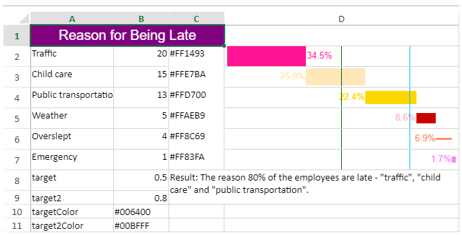
파레토 스파크라인
셀 값을 사용하여 PARETOSPARKLINE 수식을 통해 파레토 스파크라인을 추가할 수 있습니다.
파레토 스파크라인 수식에는 다음과 같은 옵션이 있습니다:
옵션 | 설명 |
|---|---|
points | 모든 값이 포함된 셀 범위를 나타내는 참조입니다. 예: |
pointIndex |
인덱스는 1 이상이어야 합니다. |
colorRange | 각 세그먼트 박스에 대한 색상이 포함된 셀 범위를 나타냅니다. 예: |
target | 첫 번째 목표선의 위치를 나타내는 숫자 또는 참조입니다. 예: 표시될 경우 선 색상은 |
target2 | 두 번째 목표선의 위치를 나타내는 숫자 또는 참조입니다. 예: 표시될 경우 선 색상은 |
highlightPosition | 빨간색으로 강조할 세그먼트의 순위를 나타내는 숫자 또는 참조입니다. 예: 예: 지정하지 않으면 |
label | 레이블 표시 형식을 지정하는 숫자입니다. (선택 사항, 기본값:
|
vertical | 박스 방향을 세로로 표시할지 여부를 나타내는 불리언 값입니다. (선택 사항, 기본값: 하나의 파레토 스파크라인 그룹에서는 모두 동일한 vertical 값을 사용해야 합니다. |
targetColor | 첫 번째 목표선의 색상을 나타내는 문자열입니다. (선택 사항) |
target2Color | 두 번째 목표선의 색상을 나타내는 문자열입니다. (선택 사항) |
labelColor | 레이블 전경색을 나타내는 문자열입니다. (선택 사항) |
barSize | 셀의 너비 또는 높이에 대한 막대의 비율을 나타내는 |
파레토 스파크라인 수식의 형식은 다음과 같습니다:
=PARETOSPARKLINE(points, pointIndex, colorRange, target, target2, hightlightPosition, lable, vertical, targetColor, target2Color, labelColor, barSize)
파레토 스파크라인은 하나의 그룹으로 작동하므로, 같은 그룹 내 모든 수식에 대해 vertical 값을 동일하게 설정해야 합니다.
두 번째 인자인 pointIndex는 points 범위 내 값의 인덱스를 참조합니다. 예를 들어, 아래 예시에서 2는 값 15를 참조합니다.
다음 코드 샘플은 여러 수식을 이용하여 파레토 스파크라인을 생성하는 예시입니다.
// Spread 초기화
var spread = new GC.Spread.Sheets.Workbook(document.getElementById('ss'), { sheetCount: 1 });
// activesheet 가져오기
var activeSheet = spread.getSheet(0);
activeSheet.addSpan(0, 0, 1, 3);
activeSheet.getCell(0, 0, GC.Spread.Sheets.SheetArea.viewport).value("Reason for Being Late")
    .font("20px Arial")
    .hAlign(GC.Spread.Sheets.HorizontalAlign.center)
    .vAlign(GC.Spread.Sheets.VerticalAlign.center)
    .backColor("purple")
    .foreColor("white");
activeSheet.getRange(1, 2, 6, 1, GC.Spread.Sheets.SheetArea.viewport).setBorder(new GC.Spread.Sheets.LineBorder("transparent", GC.Spread.Sheets.LineStyle.thin),
    { inside: true });
activeSheet.setValue(1, 0, "Traffic");
activeSheet.setValue(2, 0, "Child care");
activeSheet.setValue(3, 0, "Public transportation");
activeSheet.setValue(4, 0, "Weather");
activeSheet.setValue(5, 0, "Overslept");
activeSheet.setValue(6, 0, "Emergency");
activeSheet.setValue(7, 0, "target");
activeSheet.setValue(8, 0, "target2");
activeSheet.setValue(1, 1, 20);
activeSheet.setValue(2, 1, 15);
activeSheet.setValue(3, 1, 13);
activeSheet.setValue(4, 1, 5);
activeSheet.setValue(5, 1, 4);
activeSheet.setValue(6, 1, 1);
activeSheet.setValue(7, 1, 0.5);
activeSheet.setValue(8, 1, 0.8);
activeSheet.setValue(1, 2, "#FF1493");
activeSheet.setValue(2, 2, "#FFE7BA");
activeSheet.setValue(3, 2, "#FFD700");
activeSheet.setValue(4, 2, "#FFAEB9");
activeSheet.setValue(5, 2, "#FF8C69");
activeSheet.setValue(6, 2, "#FF83FA");
activeSheet.setValue(9, 0, "targetColor");
activeSheet.setValue(10, 0, "target2Color");
activeSheet.setValue(9, 1, "#006400");
activeSheet.setValue(10, 1, "#00BFFF");
activeSheet.addSpan(7, 2, 2, 2);
activeSheet.getCell(7, 2, GC.Spread.Sheets.SheetArea.viewport).wordWrap(true);
activeSheet.setValue(7, 2, 'Result: The reason 80% of the employees are late - "traffic", "child care" and "public transportation".');
activeSheet.setColumnWidth(0, 120);
activeSheet.setColumnWidth(1, 80);
activeSheet.setColumnWidth(2, 80);
activeSheet.setColumnWidth(3, 340);
activeSheet.setRowHeight(0, 30);
activeSheet.setRowHeight(1, 30);
activeSheet.setRowHeight(2, 30);
activeSheet.setRowHeight(3, 30);
activeSheet.setRowHeight(4, 30);
activeSheet.setRowHeight(5, 30);
activeSheet.setRowHeight(6, 30);
activeSheet.setRowHeight(7, 30);
//$B$10, $B$11, C2: C7, D2: D7
//targetColor, target2Color, labelColor, barSize)
activeSheet.setFormula(1, 3, '=PARETOSPARKLINE(B2:B7,1,C2:C7,B8,B9,4,2,false,B10,B11,C2,1)');
activeSheet.setFormula(2, 3, '=PARETOSPARKLINE(B2:B7,2,C2:C7,B8,B9,4,2,false,B10,B11,C3,0.8)');
activeSheet.setFormula(3, 3, '=PARETOSPARKLINE(B2:B7,3,C2:C7,B8,B9,4,2,false,B10,B11,C4,0.6)');
activeSheet.setFormula(4, 3, '=PARETOSPARKLINE(B2:B7,4,C2:C7,B8,B9,4,2,false,B10,B11,C5,0.5)');
activeSheet.setFormula(5, 3, '=PARETOSPARKLINE(B2:B7,5,C2:C7,B8,B9,4,2,false,B10,B11,C6,0.1)');
activeSheet.setFormula(6, 3, '=PARETOSPARKLINE(B2:B7,6,C2:C7,B8,B9,4,2,false,B10,B11,C7,0.3)');