- SpreadJS Overview
- Getting Started
- JavaScript Frameworks
- Best Practices
-
Features
- Workbook
- Worksheet
- Rows and Columns
- Headers
- Cells
- Data Binding
- TableSheet
- GanttSheet
- JSON Schema with SpreadJS
- SpreadJS File Format
- Data Validation
- Conditional Formatting
- Sort
- Group
- Formulas
- Serialization
- Keyboard Actions
- Shapes
- Form Controls
- Floating Objects
- Barcodes
- Charts
- Sparklines
- Tables
- Pivot Table
- Slicer
- Theme
- Culture
- SpreadJS Designer
- SpreadJS Designer Component
- Touch Support
- Formula Reference
- Import and Export Reference
- Frequently Used Events
- API Documentation
- Release Notes
Data Validation
SpreadJS allows users to create validators in order to validate the data input and restrict invalid information. You can display a list of valid values for the user and display an invalid data image as soon as a user enters invalid data in the cell.
You can validate the information entered in the worksheets in the following ways -
Using Different Types of Data Validation
SpreadJS provides support for the following types of data validation.
Date Validation
The createDateValidator method can be used to validate specific date criteria for a cell.
Date validation restricts users from entering invalid date information (that doesn't meet the specified date criteria for a particular cell) in the spreadsheet. For example, let's say you create a date validator to allow users to enter any date between 31st December 2017 and 31st December 2018. Any date entry outside this range will be considered an invalid data entry.
The following code sample creates a date validator.
spread.options.highlightInvalidData = true;
var dv = GC.Spread.Sheets.DataValidation.createDateValidator(GC.Spread.Sheets.ConditionalFormatting.ComparisonOperators.between, new Date(2017, 12, 31), new Date(2018, 12, 31));
dv.showInputMessage(true);
dv.inputMessage("Enter a date between 12/31/2017 and 12/31/2018.");
dv.inputTitle("Tip");
activeSheet.setDataValidator(1, 1, 1, 1, dv, GC.Spread.Sheets.SheetArea.viewport);
Formula Validation
The createFormulaValidator method can be used to validate the formula entered in a cell.
The following code sample creates a formula validator.
spread.options.highlightInvalidData = true;
//The formula validator is valid if the formula condition returns true.
var dv = GC.Spread.Sheets.DataValidation.createFormulaValidator("A1>0");
dv.showInputMessage(true);
dv.inputMessage("Enter a value greater than 0 in A1.");
dv.inputTitle("Tip");
activeSheet.setDataValidator(0, 0, 1, 1, dv, GC.Spread.Sheets.SheetArea.viewport);
Formula List Validation
The createFormulaListValidator method can be used to validate the list of formulas in the spreadsheet. The formula list validator uses a range of cells to create the list of valid values.
The formula validator is valid if the formula condition returns true. The ValidationError event occurs when the applied cell value is invalid.
The following code sample creates a list of valid values based on a range of cells specified by a formula.
activeSheet.setValue(0, 2, 5);
activeSheet.setValue(1, 2, 4);
activeSheet.setValue(2, 2, 5);

spread.options.highlightInvalidData = true;
var dv = GC.Spread.Sheets.DataValidation.createFormulaListValidator("$C$1:$C$3");
dv.showInputMessage(true);
dv.inputMessage("Pick a value from the list.");
dv.inputTitle("tip");
activeSheet.setDataValidator(1, 1, 1, 1, dv, GC.Spread.Sheets.SheetArea.viewport);
var validList = activeSheet.getDataValidator(1, 1).getValidList(sheet, 1, 1);
List Validation
The createListValidator method creates a validator based on a list.
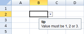
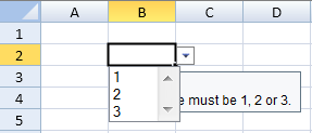
The following code sample creates a list of valid values, displays an input tip, and displays an invalid data image if the incorrect value is entered.
spread.options.highlightInvalidData = true;
var dv = GC.Spread.Sheets.DataValidation.createListValidator("1,2,3");
dv.showInputMessage(true);
dv.inputMessage("Value must be 1,2 or 3");
dv.inputTitle("tip");
activeSheet.setDataValidator(1,1,1,1,dv,GC.Spread.Sheets.SheetArea.viewport);
alert(activeSheet.getDataValidator(1,1).getValidList(activeSheet,1,1));
SpreadJS also provides support for inserting commas (via escape characters) for each paragraph in the list as shown in the below image. Cell B2 represents a list of numbers and cell D2 represents a list of operators.

The following code sample shows list validation using two different lists - one is a list of numbers and the other is a list of operators separated by commas. The two list validation criteria in different cells (B2 and D2) restrict users to choose from the values listed in the drop-down list while entering data in the cells.
// Setting column width
sheet.setColumnWidth(0, 200.0, GC.Spread.Sheets.SheetArea.viewport);
sheet.setColumnWidth(1, 120.0, GC.Spread.Sheets.SheetArea.viewport);
sheet.setColumnWidth(2, 200.0, GC.Spread.Sheets.SheetArea.viewport);
sheet.setColumnWidth(3, 120.0, GC.Spread.Sheets.SheetArea.viewport);

// Using comma in Validation Lists
var dv1 = new GC.Spread.Sheets.DataValidation.createListValidator("123\\,456,234\\,567,789\\,564");
sheet.setText(1, 0, "Choose a number from cell B2");
dv1.inputTitle("Please choose a number:");
dv1.inputMessage("Number of money");
sheet.setDataValidator(1, 1, dv1);

var dv2 = new GC.Spread.Sheets.DataValidation.createListValidator("\\,,>,<,*,/");
sheet.setText(1, 2, "Choose an operator from cell D2");
dv2.inputTitle("Please choose an operator:");
dv2.inputMessage("operator of calculator");
sheet.setDataValidator(1, 3, dv2);
Number Validation
The createNumberValidator method can be used to validate the number entered in a cell.
Number validation restricts users from entering the numeric values that fall outside the validation criteria specified for the cell.
The following code sample uses a number validator, displays an input tip, and displays an invalid data image if the incorrect value is entered.
spread.options.highlightInvalidData = true;
var dv = GC.Spread.Sheets.DataValidation.createNumberValidator(GC.Spread.Sheets.ConditionalFormatting.ComparisonOperators.between, "5", "20", true);
dv.showInputMessage(true);
dv.inputMessage("Value must be between 5 and 20.");
dv.inputTitle("tip");
activeSheet.setDataValidator(1, 1, 1, 1, dv, GC.Spread.Sheets.SheetArea.viewport);
Text Length Validation
The createTextLengthValidator method can be used to validate the length of the text entered in a cell.
You can restrict the number of characters entered in a cell using the text length validation.
The following code sample uses a text validator, displays an input tip, and displays an invalid data image if the incorrect value is entered.
spread.options.highlightInvalidData = true;
var dv = GC.Spread.Sheets.DataValidation.createTextLengthValidator(GC.Spread.Sheets.ConditionalFormatting.ComparisonOperators.greaterThan, "4", "20");
dv.showInputMessage(true);
dv.inputMessage("Number of characters must be greater than 4.");
dv.inputTitle("tip");
activeSheet.setDataValidator(1, 1, 1, 1, dv, GC.Spread.Sheets.SheetArea.viewport);
Using Different Highlight Styles for Data Validation
You can indicate invalid information in a cell using different highlight styles including the highlight type, position, color, and image. SpreadJS supports three different types of highlight types (circle, dog-ear, and icon) and six different types of highlight positions (topLeft, topRight, bottomRight, bottomLeft, outsideLeft, and outsideRight) in order to allow users to indicate invalid data in the spreadsheet. By default, the highlight type is "circle", the highlight position is topRight and the highlight color is "red". For the image in the icon highlight style, you can either specify the image URL or image base64 data.
Along with the different highlight styles, you can also show an input tip for the user and display a drop-down button that displays the list of valid values, as shown in the following images.


The highlightInvalidData property must be set to true in order to highlight the invalid information. The highlightStyle method can be used to control the style of the highlighted error with each type possessing a different style attribute.
In the image shown below, the highlight type in cell B2 represents the circle style, cell D2 represents the dog-ear style and cell F2 represents the icon style. Also, the highlight position for cell D2 is set to topLeftand cell F2 is set to outsideLeft.

The following code sample shows three different types of highlight styles - circle, dog-ear, and icon for validating data in a spreadsheet.
// Setting column width
sheet.setColumnWidth(1, 100.0, GC.Spread.Sheets.SheetArea.viewport);
sheet.setColumnWidth(3, 100.0, GC.Spread.Sheets.SheetArea.viewport);
sheet.setColumnWidth(5, 100.0, GC.Spread.Sheets.SheetArea.viewport);
// Set the option highlightInvalidData method to true
spread.options.highlightInvalidData = true;
// For circle highlightStyle
sheet.setValue(1, 1, "Juice");
var dv1 = new GC.Spread.Sheets.DataValidation.createListValidator('Fruit,Vegetable,Food');
dv1.highlightStyle({
    type: GC.Spread.Sheets.DataValidation.HighlightType.circle,
    color: 'red'
});
sheet.setDataValidator(1, 1, dv1);
// For dog-ear highlightStyle
sheet.setValue(1, 3, "Juice");
var dv2 = new GC.Spread.Sheets.DataValidation.createListValidator('Fruit,Vegetable,Food');
dv2.highlightStyle({
    type: GC.Spread.Sheets.DataValidation.HighlightType.dogEar,
    color: 'orange',
    position: GC.Spread.Sheets.DataValidation.HighlightPostition.topLeft
});
sheet.setDataValidator(1, 3, dv2);
// For icon highlightStyle
var imageData =
    "data:image/png;base64, iVBORw0KGgoAAAANSUhEUgAAACAAAAAgCAYAAABzenr0AAAC5ElEQVRYR8WXPUxTURTH//" +
    "8nbYE6YIKSCH70lcbEVOOgMTGokw7E2cVVcDQmCrzi0IFQICbGTcXVTRcDiXEiDBojmmifRCgtjYKDYsAQ0g + gx7xXadry0dfyQt / U5J57zu + c23vu /" +
    "xAWvx8td + r + OuvbhXKdEJ + AjYQcEkEGxB8KFwB8g8hLt7hGPPFg0oprljKKtGoHU8J + EblBsq6UvbEuIgmSz12UgG8m9HunPdsCCII1uifdDYp" +
    "G0m0lcLGNiKxAGPLPOgeJ4NpWPrYE + HK05wAdygiBC5UE3gQCvJXVzLXT3wcWi9c2AUyq930ZrL8BedyO4DkfInEF + 66ejPVF8v0WAIQ9gSYo + Eig2dbgG85E4" +
    "o6k69yJn0HjD2t + OYDPTXfditvxjuSpksEFSaG8L8hEeB5Ebam9IphoSCcuHZl7mCgA0FVtEGRXKQfmukjcHwt58m11VZu1fGyCQX + svycHMNXS27zqlBkrGdgEk" +
    "HSl1ny++aE58wh0b2AYwE1L2dtRgWygZ / 5ofwe / IujMqKklq03Glgr8b1ZKzNXASVVrz5CjlrO3rwLGDWhnWNUek7xVDQARecKwVxsjeLkaAICMUVcD0yB8VQEQm" +
    "WZYDayQqK8KAGSZujewDGB / FQG0CMDWqgAIItRVbRzkxXIARLAE4FHRntskGsr0M17ZNSwnyg625jWsqBHZBGA2omwrTi + WcxPsOAJDN5qtOPsYaU8BdlhObLfPc" +
    "fZBGfZHQ50mgKGESMT38jmuZfpYa / TBr5wi0r2BIQD3LFVhtxUQGfLHQt05QWL8MAaPJWfdOImzJSF2I8mATw2pRNsmSWYEnTocbFytTX2wLK1KkhYaCDDvTDjPbCl" +
    "KN0wNWb7O9dcE1TL972wuEgflij86MJNvuO1gotQor0C02QEh5QwmGwEn0OlweRq7QOktS67lEVc8muVnbV5RBX17PpwWl3678RxCEcpCbjwHX7gzjlGr4 / k / MV" +
    "GWHUHnf3sAAAAASUVORK5CYII = ";
sheet.setValue(1, 5, "Juice");
var dv3 = new GC.Spread.Sheets.DataValidation.createListValidator('Fruit,Vegetable,Food');
dv3.highlightStyle({
    type: GC.Spread.Sheets.DataValidation.HighlightType.icon,
    color: 'blue',
    position: GC.Spread.Sheets.DataValidation.HighlightPostition.outsideLeft,
    image: imageData
});
sheet.setDataValidator(1, 5, dv3);

