
- SpreadJS Overview
- Getting Started
- JavaScript Frameworks
- Best Practices
-
Features
- Workbook
- Worksheet
- Rows and Columns
- Headers
- Cells
- Data Binding
- TableSheet
- GanttSheet
- JSON Schema with SpreadJS
- SpreadJS File Format
- Data Validation
- Conditional Formatting
- Sort
- Group
- Formulas
- Serialization
- Keyboard Actions
- Shapes
- Form Controls
- Floating Objects
- Barcodes
- Charts
-
Sparklines
- Column, Line, and Winloss Sparklines with Methods
- Markers and Points
- Horizontal and Vertical Axes
- Column, Line, and Winloss Sparklines with Formulas
- Area Sparkline
- Pie Sparkline
- Scatter Sparkline
- Bullet Sparkline
- Spread Sparkline
- Stacked Sparkline
- Hbar Sparkline
- Vbar Sparkline
- Box Plot Sparkline
- Vari Sparkline
- Cascade Sparkline
- Pareto Sparkline
- Month Sparkline
- Year Sparkline
- Custom Sparkline
- Rangeblock Sparkline
- Image Sparkline
- Histogram Sparkline
- Gauge KPI Sparkline
- Tables
- Pivot Table
- Slicer
- Theme
- Culture
- SpreadJS Designer
- SpreadJS Designer Component
- Touch Support
- Formula Reference
- Import and Export Reference
- Frequently Used Events
- API Documentation
- Release Notes
Hbar Sparkline
You can create an hbar sparkline using the HBARSPARKLINE formula and cell values.
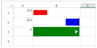
The sparkline starts at the left of the cell for positive values and the right of the cell for negative values. If the value is greater than 100% or smaller than -100%, an arrow is displayed.
The hbar sparkline has the following options:
Option | Description |
|---|---|
value | A number or reference that represents the length of the bar. The value should be between 100% and -100%. |
colorScheme | A string that represents the color of the bar. This setting is optional. The default value is "grey". |
axisVisible | A Boolean value that indicates whether or not to show the axis. Its default value is true. |
barHeight | A number greater than 0 and less than or equal to 1 to indicate the percentage of bar height according to the cell height. |
The hbar sparkline formula has the following format:
=HBARSPARKLINE(value, colorScheme, axisVisible, barHeight)
The following code sample creates hbar sparklines.
// initializing Spread
var spread = new GC.Spread.Sheets.Workbook(document.getElementById('ss'), { sheetCount: 1 });
// get the activesheet
var activeSheet = spread.getSheet(0);

activeSheet.setValue(0, 0, .3);
activeSheet.setValue(1, 0, -0.3);
activeSheet.setValue(2, 0, 2);

activeSheet.setFormula(0, 1, '=HBARSPARKLINE(A1,"red", FALSE, 0.5)');
activeSheet.setFormula(1, 1, '=HBARSPARKLINE(A2,"blue")');
activeSheet.setFormula(2, 1, '=HBARSPARKLINE(A3,"green", TRUE, A3)');

for (var i = 0; i < 4; i++) {
  activeSheet.setRowHeight(i, 40);
}
activeSheet.setColumnWidth(0, 80);
activeSheet.setColumnWidth(1, 200);