
- SpreadJS Overview
- Getting Started
- JavaScript Frameworks
- Best Practices
-
Features
- Workbook
- Worksheet
- Rows and Columns
- Headers
- Cells
- Data Binding
- TableSheet
- GanttSheet
- JSON Schema with SpreadJS
- SpreadJS File Format
- Data Validation
- Conditional Formatting
- Sort
- Group
- Formulas
- Serialization
- Keyboard Actions
- Shapes
- Form Controls
- Floating Objects
- Barcodes
- Charts
-
Sparklines
- Column, Line, and Winloss Sparklines with Methods
- Markers and Points
- Horizontal and Vertical Axes
- Column, Line, and Winloss Sparklines with Formulas
- Area Sparkline
- Pie Sparkline
- Scatter Sparkline
- Bullet Sparkline
- Spread Sparkline
- Stacked Sparkline
- Hbar Sparkline
- Vbar Sparkline
- Box Plot Sparkline
- Vari Sparkline
- Cascade Sparkline
- Pareto Sparkline
- Month Sparkline
- Year Sparkline
- Custom Sparkline
- Rangeblock Sparkline
- Image Sparkline
- Histogram Sparkline
- Gauge KPI Sparkline
- Tables
- Pivot Table
- Slicer
- Theme
- Culture
- SpreadJS Designer
- SpreadJS Designer Component
- Touch Support
- Formula Reference
- Import and Export Reference
- Frequently Used Events
- API Documentation
- Release Notes
Pie Sparkline
You can create a pie sparkline using the PIESPARKLINE formula and cell values.
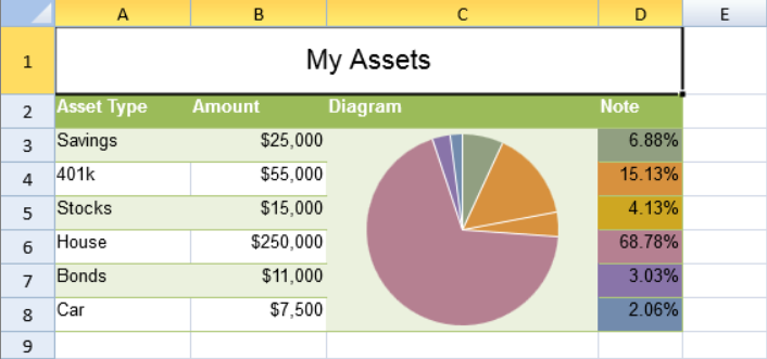
A cell value, cell range, or percent value can be used as percent values for the chart. The pie sparkline formula has percent and color options.
The pie formula has the following format:
=PIESPARKLINE(Percentage,color1,color2,.....)
If the percentage is a range (such as "A1:B3"), the percentage is the result of each cell's value divided by the sum of the range.
If the color parameter count is greater than or equal to the range count, values and colors have a one-to-two correspondence; redundant colors will be ignored. If the color parameter count is less than the range count, the given colors are reused and a linear gradient is used to ensure each section has a different color.
The following code sample creates a pie sparkline.
activeSheet.addSpan(0, 0, 1, 4);
activeSheet.getCell(0, 0, GC.Spread.Sheets.SheetArea.viewport).value("My Assets").font("20px Arial").hAlign(GC.Spread.Sheets.HorizontalAlign.center).vAlign(GC.Spread.Sheets.VerticalAlign.center);
var table1 = activeSheet.tables.add("table1", 1, 0, 7, 4, GC.Spread.Sheets.Tables.TableThemes.medium4);
table1.filterButtonVisible(false);
activeSheet.setValue(1, 0, "Asset Type");
activeSheet.setValue(1, 1, "Amount");
activeSheet.setValue(1, 2, "Diagram");
activeSheet.setValue(1, 3, "Note");
activeSheet.setValue(2, 0, "Savings");
activeSheet.setValue(2, 1, 25000);
activeSheet.setValue(3, 0, "401k");
activeSheet.setValue(3, 1, 55000);
activeSheet.setValue(4, 0, "Stocks");
activeSheet.setValue(4, 1, 15000);
activeSheet.setValue(5, 0, "House");
activeSheet.setValue(5, 1, 250000);
activeSheet.setValue(6, 0, "Bonds");
activeSheet.setValue(6, 1, 11000);
activeSheet.setValue(7, 0, "Car");
activeSheet.setValue(7, 1, 7500);
activeSheet.getRange(-1, 1, -1, 1).formatter("$#,##0");
activeSheet.addSpan(2, 2, 6, 1);
activeSheet.setFormula(2, 2, '=PIESPARKLINE(B3:B8,"#919F81","#D7913E","CEA722","#B58091","#8974A9","#728BAD")');
activeSheet.getCell(2, 3, GC.Spread.Sheets.SheetArea.viewport).backColor("#919F81").formula("=B3/SUM(B3:B8)");
activeSheet.getCell(3, 3, GC.Spread.Sheets.SheetArea.viewport).backColor("#D7913E").formula("=B4/SUM(B3:B8)");
activeSheet.getCell(4, 3, GC.Spread.Sheets.SheetArea.viewport).backColor("#CEA722").formula("=B5/SUM(B3:B8)");
activeSheet.getCell(5, 3, GC.Spread.Sheets.SheetArea.viewport).backColor("#B58091").formula("=B6/SUM(B3:B8)");
activeSheet.getCell(6, 3, GC.Spread.Sheets.SheetArea.viewport).backColor("#8974A9").formula("=B7/SUM(B3:B8)");
activeSheet.getCell(7, 3, GC.Spread.Sheets.SheetArea.viewport).backColor("#728BAD").formula("=B8/SUM(B3:B8)");
activeSheet.getCell(-1, 3).formatter("0.00%");
activeSheet.setRowHeight(0, 50);
for (var i = 1; i < 8; i++) {
    activeSheet.setRowHeight(i, 25);
}
activeSheet.setColumnWidth(0, 100);
activeSheet.setColumnWidth(1, 100);
activeSheet.setColumnWidth(2, 200);